PCM properties

The PCM class does a lot of data preprocessing under the hood in order to classify profiles.

Here is how to access PCM preprocessed results and data.

Import and set-up

Import the library and toy data

import pyxpcm
from pyxpcm.models import pcm

Let’s work with a standard PCM of temperature and salinity, from the surface down to -1000m:

# Define a vertical axis to work with
z = np.arange(0.,-1000,-10.)

# Define features to use
features_pcm = {'temperature': z, 'salinity': z}

# Instantiate the PCM
m = pcm(K=4, features=features_pcm, maxvar=2)
print(m)

<pcm 'gmm' (K: 4, F: 2)>
Number of class: 4
Number of feature: 2
Feature names: odict_keys(['temperature', 'salinity'])
Fitted: False
Feature: 'temperature'
         Interpoler: <class 'pyxpcm.utils.Vertical_Interpolator'>
         Scaler: 'normal', <class 'sklearn.preprocessing.data.StandardScaler'>
         Reducer: True, <class 'sklearn.decomposition.pca.PCA'>
Feature: 'salinity'
         Interpoler: <class 'pyxpcm.utils.Vertical_Interpolator'>
         Scaler: 'normal', <class 'sklearn.preprocessing.data.StandardScaler'>
         Reducer: True, <class 'sklearn.decomposition.pca.PCA'>
Classifier: 'gmm', <class 'sklearn.mixture.gaussian_mixture.GaussianMixture'>

Note that here we used a strong dimensionality reduction to limit the dimensions and size of the plots to come (maxvar==2 tell the PCM to use the first 2 PCAs of each variables).

Now we can load a dataset to be used for fitting.

ds = pyxpcm.tutorial.open_dataset('argo').load()

Fit and predict model on data:

features_in_ds = {'temperature': 'TEMP', 'salinity': 'PSAL'}
ds = ds.pyxpcm.fit_predict(m, features=features_in_ds, inplace=True)
print(ds)

<xarray.Dataset>
Dimensions:     (DEPTH: 282, N_PROF: 7560)
Coordinates:
  * N_PROF      (N_PROF) int64 0 1 2 3 4 5 6 ... 7554 7555 7556 7557 7558 7559
  * DEPTH       (DEPTH) float32 0.0 -5.0 -10.0 -15.0 ... -1395.0 -1400.0 -1405.0
Data variables:
    LATITUDE    (N_PROF) float32 ...
    LONGITUDE   (N_PROF) float32 ...
    TIME        (N_PROF) datetime64[ns] ...
    DBINDEX     (N_PROF) float64 ...
    TEMP        (N_PROF, DEPTH) float32 27.422163 27.422163 ... 4.391791
    PSAL        (N_PROF, DEPTH) float32 36.35267 36.35267 ... 34.910286
    SIG0        (N_PROF, DEPTH) float32 ...
    BRV2        (N_PROF, DEPTH) float32 ...
    PCM_LABELS  (N_PROF) int64 1 1 1 1 1 1 1 1 1 1 1 1 ... 3 3 3 3 3 3 3 3 3 3 3
Attributes:
    Sample test prepared by:  G. Maze
    Institution:              Ifremer/LOPS
    Data source DOI:          10.17882/42182

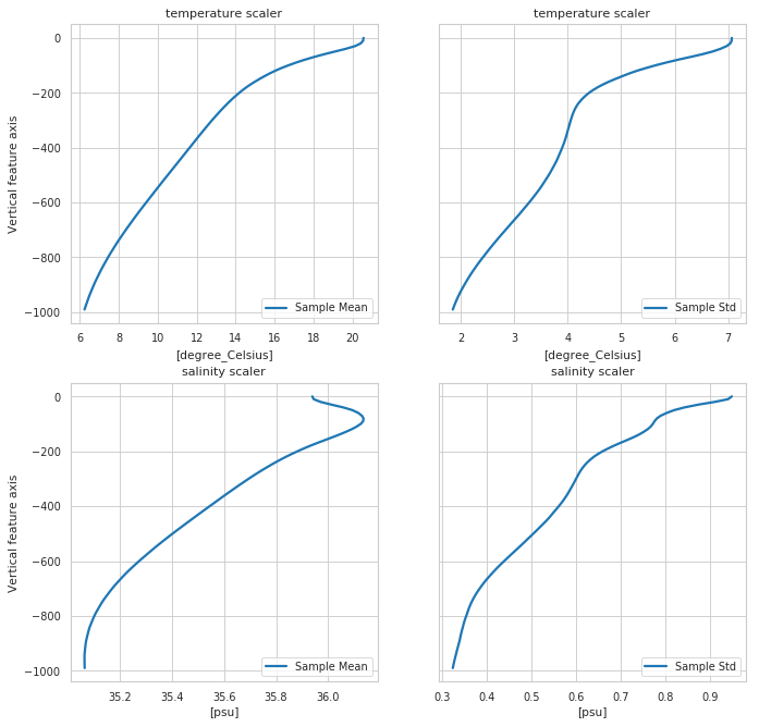
Scaler properties

fig, ax = m.plot.scaler()

# More options:
# m.plot.scaler(style='darkgrid')
# m.plot.scaler(style='darkgrid', subplot_kw={'ylim':[-1000,0]})

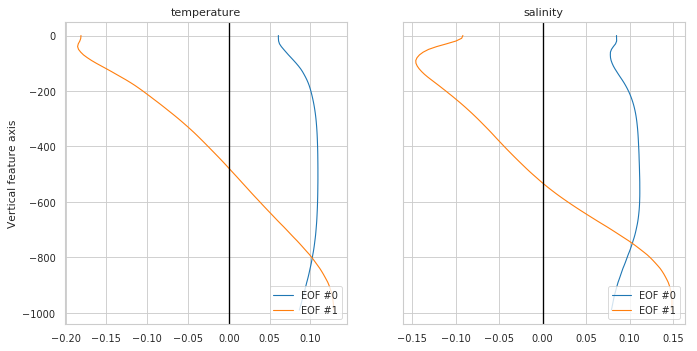
Reducer properties

Plot eigen vectors for a PCA reducer or nothing if no reduced used

fig, ax = m.plot.reducer()
# Equivalent to:
# pcmplot.reducer(m)

# More options:
# m.plot.reducer(pcalist = range(0,4));
# m.plot.reducer(pcalist = [0], maxcols=1);
# m.plot.reducer(pcalist = range(0,4), style='darkgrid',  plot_kw={'linewidth':1.5}, subplot_kw={'ylim':[-1400,0]}, figsize=(12,10));

Scatter plot of features, as seen by the classifier

You can have access to pre-processed data for your own plot/analysis through the pyxpcm.pcm.preprocessing() method:

X, sampling_dims = m.preprocessing(ds, features=features_in_ds)
X

<xarray.DataArray (n_samples: 7560, n_features: 4)>
array([[ 1.928166, -0.091499,  1.7341  , -0.270248],
       [ 2.314077,  0.106842,  2.083683, -0.18765 ],
       [ 1.675512, -0.17313 ,  1.563701, -0.432449],
       ...,
       [-0.802601, -0.578377, -1.576134, -0.311841],
       [-0.955218, -0.609439, -1.804922, -0.427322],
       [-0.892514, -0.623732, -1.792266, -0.465512]], dtype=float32)
Coordinates:
  * n_samples   (n_samples) int64 0 1 2 3 4 5 ... 7554 7555 7556 7557 7558 7559
  * n_features  (n_features) <U13 'temperature_0' ... 'salinity_1'

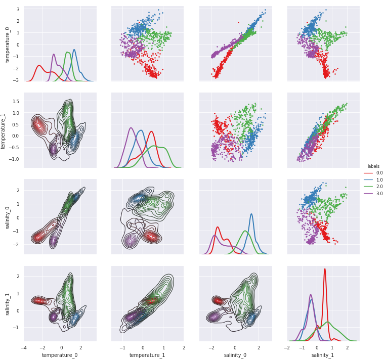
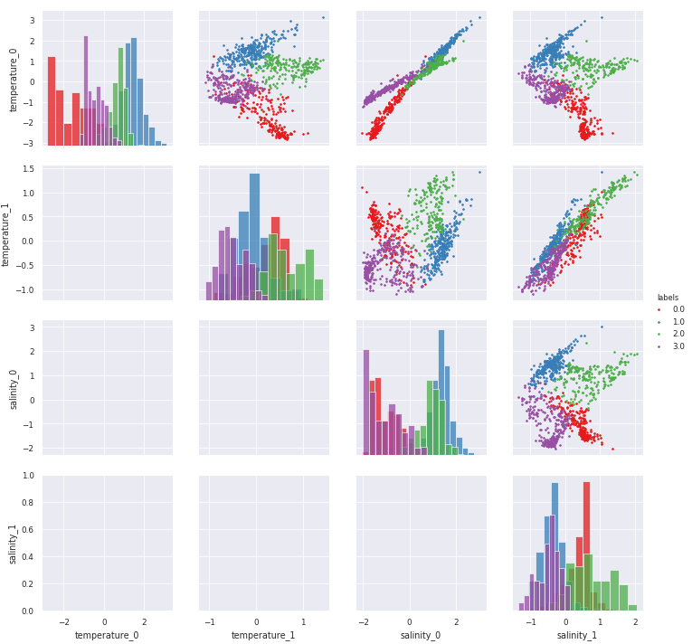
pyXpcm return a 2-dimensional xarray.DataArray for which pairwise relationship can easily be visualise with the pyxpcm.plot.preprocessed() method (this requires Seaborn):

g = m.plot.preprocessed(ds, features=features_in_ds, style='darkgrid')

# A posteriori adjustements:
# g.set(xlim=(-3,3),ylim=(-3,3))
# g.savefig('toto.png')

# Combine KDE with histrograms (very slow plot, so commented here):
g = m.plot.preprocessed(ds, features=features_in_ds, kde=True)

/Users/gmaze/anaconda/envs/obidam36/lib/python3.6/site-packages/scipy/stats/stats.py:1713: FutureWarning: Using a non-tuple sequence for multidimensional indexing is deprecated; use `arr[tuple(seq)]` instead of `arr[seq]`. In the future this will be interpreted as an array index, `arr[np.array(seq)]`, which will result either in an error or a different result.
  return np.add.reduce(sorted[indexer] * weights, axis=axis) / sumval