Standard procedure
Here is a standard procedure based on pyXpcm. This will show you how to create a model, how to fit/train it, how to classify data and to visualise results.
Create a model
Let’s import the Profile Classification Model (PCM) constructor:
[2]:
from pyxpcm.models import pcm
A PCM can be created independently of any dataset using the class constructor.
To be created a PCM requires a number of classes (or clusters) and a dictionary to define the list of features and their vertical axis:
[3]:
z = np.arange(0.,-1000,-10.)
pcm_features = {'temperature': z, 'salinity':z}
We can now instantiate a PCM, say with 8 classes:
[4]:
m = pcm(K=8, features=pcm_features)
m
[4]:
<pcm 'gmm' (K: 8, F: 2)>
Number of class: 8
Number of feature: 2
Feature names: odict_keys(['temperature', 'salinity'])
Fitted: False
Feature: 'temperature'
         Interpoler: <class 'pyxpcm.utils.Vertical_Interpolator'>
         Scaler: 'normal', <class 'sklearn.preprocessing._data.StandardScaler'>
         Reducer: True, <class 'sklearn.decomposition._pca.PCA'>
Feature: 'salinity'
         Interpoler: <class 'pyxpcm.utils.Vertical_Interpolator'>
         Scaler: 'normal', <class 'sklearn.preprocessing._data.StandardScaler'>
         Reducer: True, <class 'sklearn.decomposition._pca.PCA'>
Classifier: 'gmm', <class 'sklearn.mixture._gaussian_mixture.GaussianMixture'>
Here we created a PCM with 8 classes (K=8) and 2 features (F=2) that are temperature and salinity profiles defined between the surface and 1000m depth.
We furthermore note the list of transform methods that will be used to preprocess each of the features (see the preprocessing documentation page for more details).
Note that the number of classes and features are PCM properties accessible at pyxpcm.pcm.K and pyxpcm.pcm.F.
Load training data
pyXpcm is able to work with both gridded datasets (eg: model outputs with longitude,latitude,time dimensions) and collection of profiles (eg: Argo, XBT, CTD section profiles).
In this example, let’s import a sample of North Atlantic Argo data that come with pyxpcm.pcm:
[5]:
import pyxpcm
ds = pyxpcm.tutorial.open_dataset('argo').load()
print(ds)
<xarray.Dataset>
Dimensions:    (DEPTH: 282, N_PROF: 7560)
Coordinates:
  * DEPTH      (DEPTH) float32 0.0 -5.0 -10.0 -15.0 ... -1395.0 -1400.0 -1405.0
Dimensions without coordinates: N_PROF
Data variables:
    LATITUDE   (N_PROF) float32 ...
    LONGITUDE  (N_PROF) float32 ...
    TIME       (N_PROF) datetime64[ns] ...
    DBINDEX    (N_PROF) float64 ...
    TEMP       (N_PROF, DEPTH) float32 ...
    PSAL       (N_PROF, DEPTH) float32 ...
    SIG0       (N_PROF, DEPTH) float32 ...
    BRV2       (N_PROF, DEPTH) float32 ...
Attributes:
    Sample test prepared by:  G. Maze
    Institution:              Ifremer/LOPS
    Data source DOI:          10.17882/42182
Fit the model on data
Fitting can be done on any dataset coherent with the PCM definition, in a sense that it must have the feature variables of the PCM.
To tell the PCM model how to identify features in any xarray.Dataset, we need to provide a dictionary of variable names mapping:
[6]:
features_in_ds = {'temperature': 'TEMP', 'salinity': 'PSAL'}
which means that the PCM feature temperature is to be found in the dataset variables TEMP.
We also need to specify what is the vertical dimension of the dataset variables:
[7]:
features_zdim='DEPTH'
Now we’re ready to fit the model on the this dataset:
[8]:
m.fit(ds, features=features_in_ds, dim=features_zdim)
m
[8]:
<pcm 'gmm' (K: 8, F: 2)>
Number of class: 8
Number of feature: 2
Feature names: odict_keys(['temperature', 'salinity'])
Fitted: True
Feature: 'temperature'
         Interpoler: <class 'pyxpcm.utils.Vertical_Interpolator'>
         Scaler: 'normal', <class 'sklearn.preprocessing._data.StandardScaler'>
         Reducer: True, <class 'sklearn.decomposition._pca.PCA'>
Feature: 'salinity'
         Interpoler: <class 'pyxpcm.utils.Vertical_Interpolator'>
         Scaler: 'normal', <class 'sklearn.preprocessing._data.StandardScaler'>
         Reducer: True, <class 'sklearn.decomposition._pca.PCA'>
Classifier: 'gmm', <class 'sklearn.mixture._gaussian_mixture.GaussianMixture'>
         log likelihood of the training set: 38.784750
Note
pyXpcm can also identify PCM features and axis within a xarray.DataSet with variable attributes. From the example above we can set:
ds['TEMP'].attrs['feature_name'] = 'temperature'
ds['PSAL'].attrs['feature_name'] = 'salinity'
ds['DEPTH'].attrs['axis'] = 'Z'
And then simply call the fit method without arguments:
m.fit(ds)
Note that if data follows the CF the vertical dimension axis attribute should already be set to Z.
Classify data
Now that the PCM is fitted, we can predict the classification results like:
[9]:
m.predict(ds, features=features_in_ds, inplace=True)
ds
[9]:
- DEPTH: 282
- N_PROF: 7560
- N_PROF(N_PROF)int640 1 2 3 4 ... 7556 7557 7558 7559
array([ 0, 1, 2, ..., 7557, 7558, 7559])
- DEPTH(DEPTH)float320.0 -5.0 -10.0 ... -1400.0 -1405.0
- axis :
- Z
- standard_name :
- depth
- long_name :
- Vertical Distance Below the Surface
- convention :
- Negative, downward oriented
- units :
- meters
- positive :
- up
array([ 0., -5., -10., ..., -1395., -1400., -1405.], dtype=float32)
- LATITUDE(N_PROF)float32...
- axis :
- Y
- standard_name :
- latitude
- long_name :
- Latitude
- units :
- degrees_north
array([27.122, 27.818, 27.452, ..., 4.243, 4.15 , 4.44 ], dtype=float32)
- LONGITUDE(N_PROF)float32...
- axis :
- X
- standard_name :
- longitude
- long_name :
- Longitude
- units :
- degrees_east
array([-7.4860e+01, -7.5600e+01, -7.4949e+01, ..., -1.2630e+00, -8.2100e-01, -2.0000e-03], dtype=float32) - TIME(N_PROF)datetime64[ns]...
- standard_name :
- time
- short_name :
- time
- long_name :
- Time of Measurement
array(['2008-06-23T13:07:30.000000000', '2011-05-22T12:46:24.375000064', '2011-07-11T12:54:50.624999936', ..., '2014-03-17T05:44:31.875000064', '2014-03-27T03:05:37.500000000', '2013-03-09T14:52:58.124999936'], dtype='datetime64[ns]') - DBINDEX(N_PROF)float64...
- short_name :
- index
- long_name :
- Profile index within the complete database
array([14840., 16215., 16220., ..., 8556., 8557., 10628.])
- TEMP(N_PROF, DEPTH)float3227.422163 27.422163 ... 4.391791
- long_name :
- Sea Temperature In-Situ ITS-90 Scale
- standard_name :
- sea_water_temperature
- units :
- degree_Celsius
- valid_min :
- -2.5.f
- valid_max :
- 40.f
- C_format :
- %9.3f
- FORTRAN_format :
- F9.3
- resolution :
- 0.001f
array([[27.422163, 27.422163, 27.29007 , ..., 4.436046, 4.423681, 4.411316], [25.129957, 25.129957, 24.970064, ..., 4.757417, 4.743126, 4.728835], [28.132914, 28.132914, 27.969038, ..., 4.371902, 4.356699, 4.341496], ..., [28.722956, 28.722956, 28.721252, ..., 4.275817, 4.270741, 4.266666], [28.643309, 28.643309, 28.64578 , ..., 4.292866, 4.285667, 4.278265], [29.249382, 29.249382, 29.13765 , ..., 4.412214, 4.403805, 4.391791]], dtype=float32) - PSAL(N_PROF, DEPTH)float3236.35267 36.35267 ... 34.910286
- long_name :
- Practical Salinity
- standard_name :
- sea_water_salinity
- units :
- psu
- valid_min :
- 2.f
- valid_max :
- 41.f
- C_format :
- %9.3f
- FORTRAN_format :
- F9.3
- resolution :
- 0.001f
array([[36.35267 , 36.35267 , 36.468353, ..., 35.01112 , 35.010513, 35.009903], [36.508953, 36.508953, 36.502014, ..., 35.029182, 35.02817 , 35.027157], [36.492146, 36.492146, 36.514534, ..., 34.995472, 34.994053, 34.992634], ..., [34.973022, 34.973022, 34.973873, ..., 34.92445 , 34.925774, 34.92674 ], [35.184 , 35.184 , 35.184 , ..., 34.931606, 34.933006, 34.934402], [35.05187 , 35.05187 , 35.05117 , ..., 34.9081 , 34.909523, 34.910286]], dtype=float32) - SIG0(N_PROF, DEPTH)float32...
- standard_name :
- sea_water_density
- long_name :
- Potential Density Referenced to Surface
- units :
- kg/m^3
[2131920 values with dtype=float32]
- BRV2(N_PROF, DEPTH)float32...
- standard_name :
- N2
- long_name :
- Brunt-Vaisala Frequency Squared
- units :
- 1/s^2
[2131920 values with dtype=float32]
- PCM_LABELS(N_PROF)int641 1 1 1 1 1 1 1 ... 3 3 3 3 3 3 3 3
- long_name :
- PCM labels
- units :
- valid_min :
- 0
- valid_max :
- 7
- llh :
- 38.784750479707895
- _pyXpcm_cleanable :
- 1
array([1, 1, 1, ..., 3, 3, 3])
- Sample test prepared by :
- G. Maze
- Institution :
- Ifremer/LOPS
- Data source DOI :
- 10.17882/42182
Prediction labels are automatically added to the dataset as PCM_LABELS because the option inplace was set to True. We didn’t specify the dim option because our dataset is CF compliant.
pyXpcm use a GMM classifier by default, which is a fuzzy classifier. So we can also predict the probability of each classes for all profiles, the so-called posteriors:
[10]:
m.predict_proba(ds, features=features_in_ds, inplace=True)
ds
[10]:
- DEPTH: 282
- N_PROF: 7560
- pcm_class: 8
- N_PROF(N_PROF)int640 1 2 3 4 ... 7556 7557 7558 7559
array([ 0, 1, 2, ..., 7557, 7558, 7559])
- DEPTH(DEPTH)float320.0 -5.0 -10.0 ... -1400.0 -1405.0
- axis :
- Z
- standard_name :
- depth
- long_name :
- Vertical Distance Below the Surface
- convention :
- Negative, downward oriented
- units :
- meters
- positive :
- up
array([ 0., -5., -10., ..., -1395., -1400., -1405.], dtype=float32)
- LATITUDE(N_PROF)float3227.122 27.818 27.452 ... 4.15 4.44
- axis :
- Y
- standard_name :
- latitude
- long_name :
- Latitude
- units :
- degrees_north
array([27.122, 27.818, 27.452, ..., 4.243, 4.15 , 4.44 ], dtype=float32)
- LONGITUDE(N_PROF)float32-74.86 -75.6 ... -0.821 -0.002
- axis :
- X
- standard_name :
- longitude
- long_name :
- Longitude
- units :
- degrees_east
array([-7.4860e+01, -7.5600e+01, -7.4949e+01, ..., -1.2630e+00, -8.2100e-01, -2.0000e-03], dtype=float32) - TIME(N_PROF)datetime64[ns]2008-06-23T13:07:30 ... 2013-03-09T14:52:58.124999936
- standard_name :
- time
- short_name :
- time
- long_name :
- Time of Measurement
array(['2008-06-23T13:07:30.000000000', '2011-05-22T12:46:24.375000064', '2011-07-11T12:54:50.624999936', ..., '2014-03-17T05:44:31.875000064', '2014-03-27T03:05:37.500000000', '2013-03-09T14:52:58.124999936'], dtype='datetime64[ns]') - DBINDEX(N_PROF)float641.484e+04 1.622e+04 ... 1.063e+04
- short_name :
- index
- long_name :
- Profile index within the complete database
array([14840., 16215., 16220., ..., 8556., 8557., 10628.])
- TEMP(N_PROF, DEPTH)float3227.422163 27.422163 ... 4.391791
- long_name :
- Sea Temperature In-Situ ITS-90 Scale
- standard_name :
- sea_water_temperature
- units :
- degree_Celsius
- valid_min :
- -2.5.f
- valid_max :
- 40.f
- C_format :
- %9.3f
- FORTRAN_format :
- F9.3
- resolution :
- 0.001f
array([[27.422163, 27.422163, 27.29007 , ..., 4.436046, 4.423681, 4.411316], [25.129957, 25.129957, 24.970064, ..., 4.757417, 4.743126, 4.728835], [28.132914, 28.132914, 27.969038, ..., 4.371902, 4.356699, 4.341496], ..., [28.722956, 28.722956, 28.721252, ..., 4.275817, 4.270741, 4.266666], [28.643309, 28.643309, 28.64578 , ..., 4.292866, 4.285667, 4.278265], [29.249382, 29.249382, 29.13765 , ..., 4.412214, 4.403805, 4.391791]], dtype=float32) - PSAL(N_PROF, DEPTH)float3236.35267 36.35267 ... 34.910286
- long_name :
- Practical Salinity
- standard_name :
- sea_water_salinity
- units :
- psu
- valid_min :
- 2.f
- valid_max :
- 41.f
- C_format :
- %9.3f
- FORTRAN_format :
- F9.3
- resolution :
- 0.001f
array([[36.35267 , 36.35267 , 36.468353, ..., 35.01112 , 35.010513, 35.009903], [36.508953, 36.508953, 36.502014, ..., 35.029182, 35.02817 , 35.027157], [36.492146, 36.492146, 36.514534, ..., 34.995472, 34.994053, 34.992634], ..., [34.973022, 34.973022, 34.973873, ..., 34.92445 , 34.925774, 34.92674 ], [35.184 , 35.184 , 35.184 , ..., 34.931606, 34.933006, 34.934402], [35.05187 , 35.05187 , 35.05117 , ..., 34.9081 , 34.909523, 34.910286]], dtype=float32) - SIG0(N_PROF, DEPTH)float32...
- standard_name :
- sea_water_density
- long_name :
- Potential Density Referenced to Surface
- units :
- kg/m^3
[2131920 values with dtype=float32]
- BRV2(N_PROF, DEPTH)float32...
- standard_name :
- N2
- long_name :
- Brunt-Vaisala Frequency Squared
- units :
- 1/s^2
[2131920 values with dtype=float32]
- PCM_LABELS(N_PROF)int641 1 1 1 1 1 1 1 ... 3 3 3 3 3 3 3 3
- long_name :
- PCM labels
- units :
- valid_min :
- 0
- valid_max :
- 7
- llh :
- 38.784750479707895
- _pyXpcm_cleanable :
- 1
array([1, 1, 1, ..., 3, 3, 3])
- PCM_POST(pcm_class, N_PROF)float640.0 0.0 0.0 ... 1.388e-19 6.625e-20
- long_name :
- PCM posteriors
- units :
- valid_min :
- 0
- valid_max :
- 1
- llh :
- 38.784750479707895
- _pyXpcm_cleanable :
- 1
array([[0.00000000e+000, 0.00000000e+000, 0.00000000e+000, ...,
        0.00000000e+000, 0.00000000e+000, 0.00000000e+000],
       [1.00000000e+000, 1.00000000e+000, 1.00000000e+000, ...,
        0.00000000e+000, 0.00000000e+000, 0.00000000e+000],
       [2.75142938e-035, 1.71775866e-048, 1.47313441e-051, ...,
        9.86880534e-065, 3.81613835e-035, 1.17629638e-060],
       ...,
       [3.62174559e-041, 1.53234929e-041, 2.04866455e-011, ...,
        3.58739580e-156, 7.71107953e-076, 5.77624573e-087],
       [1.75054380e-043, 4.39827507e-058, 9.91303461e-043, ...,
        0.00000000e+000, 2.51971559e-279, 0.00000000e+000],
       [1.51181396e-037, 2.06372255e-057, 1.60024100e-030, ...,
        1.09259071e-008, 1.38768016e-019, 6.62479874e-020]])
- Sample test prepared by :
- G. Maze
- Institution :
- Ifremer/LOPS
- Data source DOI :
- 10.17882/42182
which are added to the dataset as the PCM_POST variables. The probability of classes for each profiles has a new dimension pcm_class by default that goes from 0 to K-1.
Note
You can delete variables added by pyXpcm to the xarray.DataSet with the pyxpcm.xarray.pyXpcmDataSetAccessor.drop_all() method:
ds.pyxpcm.drop_all()
Or you can split pyXpcm variables out of the original xarray.DataSet:
ds_pcm, ds = ds.pyxpcm.split()
It is important to note that once the PCM is fitted, you can predict labels for any dataset, as long as it has the PCM features.
For instance, let’s predict labels for a gridded dataset:
[12]:
ds_gridded = pyxpcm.tutorial.open_dataset('isas_snapshot').load()
ds_gridded
[12]:
- depth: 152
- latitude: 53
- longitude: 61
- latitude(latitude)float3230.023445 30.455408 ... 49.737103
- standard_name :
- latitude
- units :
- degree_north
- valid_min :
- -90.0
- valid_max :
- 90.0
- axis :
- Y
array([30.023445, 30.455408, 30.885464, 31.313599, 31.739796, 32.16404 , 32.58632 , 33.006615, 33.424923, 33.84122 , 34.2555 , 34.66775 , 35.07796 , 35.48612 , 35.892216, 36.296238, 36.698177, 37.09803 , 37.49578 , 37.891426, 38.284954, 38.67636 , 39.06564 , 39.452785, 39.837788, 40.220642, 40.60135 , 40.979897, 41.35629 , 41.73051 , 42.10257 , 42.472458, 42.84017 , 43.20571 , 43.569073, 43.930252, 44.289257, 44.646076, 45.000717, 45.353176, 45.703453, 46.051548, 46.39746 , 46.7412 , 47.08276 , 47.422142, 47.75935 , 48.094387, 48.427258, 48.757957, 49.0865 , 49.41288 , 49.737103], dtype=float32) - longitude(longitude)float32-70.0 -69.5 -69.0 ... -40.5 -40.0
- standard_name :
- longitude
- units :
- degree_east
- valid_min :
- -180.0
- valid_max :
- 180.0
- axis :
- X
array([-70. , -69.5, -69. , -68.5, -68. , -67.5, -67. , -66.5, -66. , -65.5, -65. , -64.5, -64. , -63.5, -63. , -62.5, -62. , -61.5, -61. , -60.5, -60. , -59.5, -59. , -58.5, -58. , -57.5, -57. , -56.5, -56. , -55.5, -55. , -54.5, -54. , -53.5, -53. , -52.5, -52. , -51.5, -51. , -50.5, -50. , -49.5, -49. , -48.5, -48. , -47.5, -47. , -46.5, -46. , -45.5, -45. , -44.5, -44. , -43.5, -43. , -42.5, -42. , -41.5, -41. , -40.5, -40. ], dtype=float32) - depth(depth)float32-1.0 -3.0 -5.0 ... -1980.0 -2000.0
- axis :
- Z
- units :
- meters
- positive :
- up
array([-1.00e+00, -3.00e+00, -5.00e+00, -1.00e+01, -1.50e+01, -2.00e+01,
       -2.50e+01, -3.00e+01, -3.50e+01, -4.00e+01, -4.50e+01, -5.00e+01,
       -5.50e+01, -6.00e+01, -6.50e+01, -7.00e+01, -7.50e+01, -8.00e+01,
       -8.50e+01, -9.00e+01, -9.50e+01, -1.00e+02, -1.10e+02, -1.20e+02,
       -1.30e+02, -1.40e+02, -1.50e+02, -1.60e+02, -1.70e+02, -1.80e+02,
       -1.90e+02, -2.00e+02, -2.10e+02, -2.20e+02, -2.30e+02, -2.40e+02,
       -2.50e+02, -2.60e+02, -2.70e+02, -2.80e+02, -2.90e+02, -3.00e+02,
       -3.10e+02, -3.20e+02, -3.30e+02, -3.40e+02, -3.50e+02, -3.60e+02,
       -3.70e+02, -3.80e+02, -3.90e+02, -4.00e+02, -4.10e+02, -4.20e+02,
       -4.30e+02, -4.40e+02, -4.50e+02, -4.60e+02, -4.70e+02, -4.80e+02,
       -4.90e+02, -5.00e+02, -5.10e+02, -5.20e+02, -5.30e+02, -5.40e+02,
       -5.50e+02, -5.60e+02, -5.70e+02, -5.80e+02, -5.90e+02, -6.00e+02,
       -6.10e+02, -6.20e+02, -6.30e+02, -6.40e+02, -6.50e+02, -6.60e+02,
       -6.70e+02, -6.80e+02, -6.90e+02, -7.00e+02, -7.10e+02, -7.20e+02,
       -7.30e+02, -7.40e+02, -7.50e+02, -7.60e+02, -7.70e+02, -7.80e+02,
       -7.90e+02, -8.00e+02, -8.20e+02, -8.40e+02, -8.60e+02, -8.80e+02,
       -9.00e+02, -9.20e+02, -9.40e+02, -9.60e+02, -9.80e+02, -1.00e+03,
       -1.02e+03, -1.04e+03, -1.06e+03, -1.08e+03, -1.10e+03, -1.12e+03,
       -1.14e+03, -1.16e+03, -1.18e+03, -1.20e+03, -1.22e+03, -1.24e+03,
       -1.26e+03, -1.28e+03, -1.30e+03, -1.32e+03, -1.34e+03, -1.36e+03,
       -1.38e+03, -1.40e+03, -1.42e+03, -1.44e+03, -1.46e+03, -1.48e+03,
       -1.50e+03, -1.52e+03, -1.54e+03, -1.56e+03, -1.58e+03, -1.60e+03,
       -1.62e+03, -1.64e+03, -1.66e+03, -1.68e+03, -1.70e+03, -1.72e+03,
       -1.74e+03, -1.76e+03, -1.78e+03, -1.80e+03, -1.82e+03, -1.84e+03,
       -1.86e+03, -1.88e+03, -1.90e+03, -1.92e+03, -1.94e+03, -1.96e+03,
       -1.98e+03, -2.00e+03], dtype=float32)
- TEMP(depth, latitude, longitude)float32dask.array<chunksize=(152, 53, 61), meta=np.ndarray>
- long_name :
- Temperature
- standard_name :
- sea_water_temperature
- units :
- degree_Celsius
- valid_min :
- -23000
- valid_max :
- 20000
Array Chunk Bytes 1.97 MB 1.97 MB Shape (152, 53, 61) (152, 53, 61) Count 2 Tasks 1 Chunks Type float32 numpy.ndarray - TEMP_ERR(depth, latitude, longitude)float32dask.array<chunksize=(152, 53, 61), meta=np.ndarray>
- long_name :
- Temperature Error
- standard_name :
- units :
- degree_Celsius
- valid_min :
- 0
- valid_max :
- 20000
Array Chunk Bytes 1.97 MB 1.97 MB Shape (152, 53, 61) (152, 53, 61) Count 2 Tasks 1 Chunks Type float32 numpy.ndarray - TEMP_PCTVAR(depth, latitude, longitude)float32dask.array<chunksize=(152, 53, 61), meta=np.ndarray>
- long_name :
- Error on TEMP variable (% variance)
- standard_name :
- units :
- %
- valid_min :
- 0.0
- valid_max :
- 100.0
Array Chunk Bytes 1.97 MB 1.97 MB Shape (152, 53, 61) (152, 53, 61) Count 2 Tasks 1 Chunks Type float32 numpy.ndarray - PSAL(depth, latitude, longitude)float32dask.array<chunksize=(152, 53, 61), meta=np.ndarray>
- long_name :
- Practical salinity
- standard_name :
- sea_water_salinity
- units :
- PSS-78
- valid_min :
- -26000
- valid_max :
- 30000
Array Chunk Bytes 1.97 MB 1.97 MB Shape (152, 53, 61) (152, 53, 61) Count 2 Tasks 1 Chunks Type float32 numpy.ndarray - PSAL_ERR(depth, latitude, longitude)float32dask.array<chunksize=(152, 53, 61), meta=np.ndarray>
- long_name :
- Practical salinity Error
- standard_name :
- units :
- PSS-78
- valid_min :
- 0
- valid_max :
- 15000
Array Chunk Bytes 1.97 MB 1.97 MB Shape (152, 53, 61) (152, 53, 61) Count 2 Tasks 1 Chunks Type float32 numpy.ndarray - PSAL_PCTVAR(depth, latitude, longitude)float32dask.array<chunksize=(152, 53, 61), meta=np.ndarray>
- long_name :
- Error on PSAL variable (% variance)
- standard_name :
- units :
- %
- valid_min :
- 0.0
- valid_max :
- 100.0
Array Chunk Bytes 1.97 MB 1.97 MB Shape (152, 53, 61) (152, 53, 61) Count 2 Tasks 1 Chunks Type float32 numpy.ndarray - SST(latitude, longitude)float32dask.array<chunksize=(53, 61), meta=np.ndarray>
- long_name :
- Temperature
- standard_name :
- sea_water_temperature
- units :
- degree_Celsius
- valid_min :
- -23000
- valid_max :
- 20000
Array Chunk Bytes 12.93 kB 12.93 kB Shape (53, 61) (53, 61) Count 2 Tasks 1 Chunks Type float32 numpy.ndarray
[13]:
m.predict(ds_gridded, features={'temperature':'TEMP','salinity':'PSAL'}, dim='depth', inplace=True)
ds_gridded
[13]:
- depth: 152
- latitude: 53
- longitude: 61
- latitude(latitude)float6430.02 30.46 30.89 ... 49.41 49.74
array([30.023445, 30.455408, 30.885464, 31.313599, 31.739796, 32.16404 , 32.586319, 33.006615, 33.424923, 33.841221, 34.255501, 34.667751, 35.077961, 35.486118, 35.892216, 36.296238, 36.698177, 37.09803 , 37.495781, 37.891426, 38.284954, 38.676361, 39.065639, 39.452785, 39.837788, 40.220642, 40.601349, 40.979897, 41.356289, 41.730511, 42.10257 , 42.472458, 42.840172, 43.205711, 43.569073, 43.930252, 44.289257, 44.646076, 45.000717, 45.353176, 45.703453, 46.051548, 46.397461, 46.741199, 47.08276 , 47.422142, 47.75935 , 48.094387, 48.427258, 48.757957, 49.086498, 49.41288 , 49.737103]) - longitude(longitude)float64-70.0 -69.5 -69.0 ... -40.5 -40.0
array([-70. , -69.5, -69. , -68.5, -68. , -67.5, -67. , -66.5, -66. , -65.5, -65. , -64.5, -64. , -63.5, -63. , -62.5, -62. , -61.5, -61. , -60.5, -60. , -59.5, -59. , -58.5, -58. , -57.5, -57. , -56.5, -56. , -55.5, -55. , -54.5, -54. , -53.5, -53. , -52.5, -52. , -51.5, -51. , -50.5, -50. , -49.5, -49. , -48.5, -48. , -47.5, -47. , -46.5, -46. , -45.5, -45. , -44.5, -44. , -43.5, -43. , -42.5, -42. , -41.5, -41. , -40.5, -40. ]) - depth(depth)float32-1.0 -3.0 -5.0 ... -1980.0 -2000.0
- axis :
- Z
- units :
- meters
- positive :
- up
array([-1.00e+00, -3.00e+00, -5.00e+00, -1.00e+01, -1.50e+01, -2.00e+01,
       -2.50e+01, -3.00e+01, -3.50e+01, -4.00e+01, -4.50e+01, -5.00e+01,
       -5.50e+01, -6.00e+01, -6.50e+01, -7.00e+01, -7.50e+01, -8.00e+01,
       -8.50e+01, -9.00e+01, -9.50e+01, -1.00e+02, -1.10e+02, -1.20e+02,
       -1.30e+02, -1.40e+02, -1.50e+02, -1.60e+02, -1.70e+02, -1.80e+02,
       -1.90e+02, -2.00e+02, -2.10e+02, -2.20e+02, -2.30e+02, -2.40e+02,
       -2.50e+02, -2.60e+02, -2.70e+02, -2.80e+02, -2.90e+02, -3.00e+02,
       -3.10e+02, -3.20e+02, -3.30e+02, -3.40e+02, -3.50e+02, -3.60e+02,
       -3.70e+02, -3.80e+02, -3.90e+02, -4.00e+02, -4.10e+02, -4.20e+02,
       -4.30e+02, -4.40e+02, -4.50e+02, -4.60e+02, -4.70e+02, -4.80e+02,
       -4.90e+02, -5.00e+02, -5.10e+02, -5.20e+02, -5.30e+02, -5.40e+02,
       -5.50e+02, -5.60e+02, -5.70e+02, -5.80e+02, -5.90e+02, -6.00e+02,
       -6.10e+02, -6.20e+02, -6.30e+02, -6.40e+02, -6.50e+02, -6.60e+02,
       -6.70e+02, -6.80e+02, -6.90e+02, -7.00e+02, -7.10e+02, -7.20e+02,
       -7.30e+02, -7.40e+02, -7.50e+02, -7.60e+02, -7.70e+02, -7.80e+02,
       -7.90e+02, -8.00e+02, -8.20e+02, -8.40e+02, -8.60e+02, -8.80e+02,
       -9.00e+02, -9.20e+02, -9.40e+02, -9.60e+02, -9.80e+02, -1.00e+03,
       -1.02e+03, -1.04e+03, -1.06e+03, -1.08e+03, -1.10e+03, -1.12e+03,
       -1.14e+03, -1.16e+03, -1.18e+03, -1.20e+03, -1.22e+03, -1.24e+03,
       -1.26e+03, -1.28e+03, -1.30e+03, -1.32e+03, -1.34e+03, -1.36e+03,
       -1.38e+03, -1.40e+03, -1.42e+03, -1.44e+03, -1.46e+03, -1.48e+03,
       -1.50e+03, -1.52e+03, -1.54e+03, -1.56e+03, -1.58e+03, -1.60e+03,
       -1.62e+03, -1.64e+03, -1.66e+03, -1.68e+03, -1.70e+03, -1.72e+03,
       -1.74e+03, -1.76e+03, -1.78e+03, -1.80e+03, -1.82e+03, -1.84e+03,
       -1.86e+03, -1.88e+03, -1.90e+03, -1.92e+03, -1.94e+03, -1.96e+03,
       -1.98e+03, -2.00e+03], dtype=float32)
- TEMP(depth, latitude, longitude)float32dask.array<chunksize=(152, 53, 61), meta=np.ndarray>
- long_name :
- Temperature
- standard_name :
- sea_water_temperature
- units :
- degree_Celsius
- valid_min :
- -23000
- valid_max :
- 20000
Array Chunk Bytes 1.97 MB 1.97 MB Shape (152, 53, 61) (152, 53, 61) Count 2 Tasks 1 Chunks Type float32 numpy.ndarray - TEMP_ERR(depth, latitude, longitude)float32dask.array<chunksize=(152, 53, 61), meta=np.ndarray>
- long_name :
- Temperature Error
- standard_name :
- units :
- degree_Celsius
- valid_min :
- 0
- valid_max :
- 20000
Array Chunk Bytes 1.97 MB 1.97 MB Shape (152, 53, 61) (152, 53, 61) Count 2 Tasks 1 Chunks Type float32 numpy.ndarray - TEMP_PCTVAR(depth, latitude, longitude)float32dask.array<chunksize=(152, 53, 61), meta=np.ndarray>
- long_name :
- Error on TEMP variable (% variance)
- standard_name :
- units :
- %
- valid_min :
- 0.0
- valid_max :
- 100.0
Array Chunk Bytes 1.97 MB 1.97 MB Shape (152, 53, 61) (152, 53, 61) Count 2 Tasks 1 Chunks Type float32 numpy.ndarray - PSAL(depth, latitude, longitude)float32dask.array<chunksize=(152, 53, 61), meta=np.ndarray>
- long_name :
- Practical salinity
- standard_name :
- sea_water_salinity
- units :
- PSS-78
- valid_min :
- -26000
- valid_max :
- 30000
Array Chunk Bytes 1.97 MB 1.97 MB Shape (152, 53, 61) (152, 53, 61) Count 2 Tasks 1 Chunks Type float32 numpy.ndarray - PSAL_ERR(depth, latitude, longitude)float32dask.array<chunksize=(152, 53, 61), meta=np.ndarray>
- long_name :
- Practical salinity Error
- standard_name :
- units :
- PSS-78
- valid_min :
- 0
- valid_max :
- 15000
Array Chunk Bytes 1.97 MB 1.97 MB Shape (152, 53, 61) (152, 53, 61) Count 2 Tasks 1 Chunks Type float32 numpy.ndarray - PSAL_PCTVAR(depth, latitude, longitude)float32dask.array<chunksize=(152, 53, 61), meta=np.ndarray>
- long_name :
- Error on PSAL variable (% variance)
- standard_name :
- units :
- %
- valid_min :
- 0.0
- valid_max :
- 100.0
Array Chunk Bytes 1.97 MB 1.97 MB Shape (152, 53, 61) (152, 53, 61) Count 2 Tasks 1 Chunks Type float32 numpy.ndarray - SST(latitude, longitude)float32dask.array<chunksize=(53, 61), meta=np.ndarray>
- long_name :
- Temperature
- standard_name :
- sea_water_temperature
- units :
- degree_Celsius
- valid_min :
- -23000
- valid_max :
- 20000
Array Chunk Bytes 12.93 kB 12.93 kB Shape (53, 61) (53, 61) Count 2 Tasks 1 Chunks Type float32 numpy.ndarray - PCM_LABELS(latitude, longitude)float641.0 1.0 1.0 1.0 ... 7.0 7.0 7.0 7.0
- long_name :
- PCM labels
- units :
- valid_min :
- 0
- valid_max :
- 7
- llh :
- 37.003444293299125
- _pyXpcm_cleanable :
- 1
array([[ 1.,  1.,  1., ...,  6.,  6.,  6.],
       [ 1.,  1.,  1., ...,  6.,  6.,  6.],
       [ 1.,  1.,  1., ...,  6.,  6.,  6.],
       ...,
       [nan, nan, nan, ...,  7.,  7.,  7.],
       [nan, nan, nan, ...,  7.,  7.,  7.],
       [nan, nan, nan, ...,  7.,  7.,  7.]])
where you can see the adition of the PCM_LABELS variable.
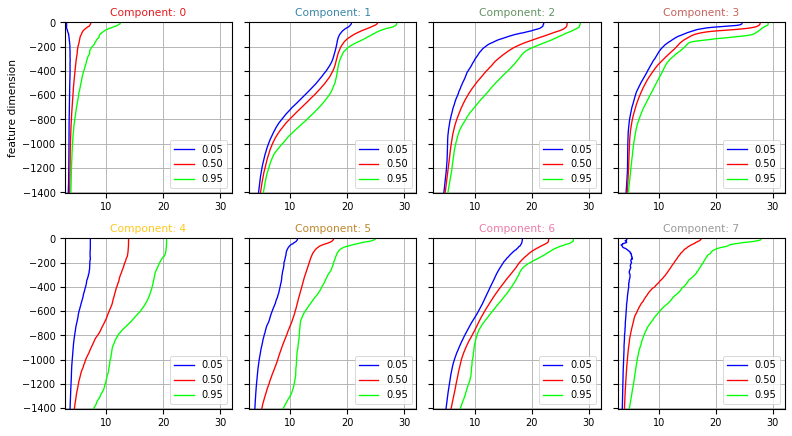
Vertical structure of classes
One key outcome of the PCM analysis if the vertical structure of each classes.
This can be computed using the :meth:pyxpcm.stat.quantile method.
Below we compute the 5, 50 and 95% quantiles for temperature and salinity of each classes:
[14]:
for vname in ['TEMP', 'PSAL']:
    ds = ds.pyxpcm.quantile(m, q=[0.05, 0.5, 0.95], of=vname, outname=vname + '_Q', keep_attrs=True, inplace=True)
ds
[14]:
- DEPTH: 282
- N_PROF: 7560
- pcm_class: 8
- quantile: 3
- pcm_class(pcm_class)int640 1 2 3 4 5 6 7
array([0, 1, 2, 3, 4, 5, 6, 7])
- N_PROF(N_PROF)int640 1 2 3 4 ... 7556 7557 7558 7559
array([ 0, 1, 2, ..., 7557, 7558, 7559])
- DEPTH(DEPTH)float320.0 -5.0 -10.0 ... -1400.0 -1405.0
- axis :
- Z
- standard_name :
- depth
- long_name :
- Vertical Distance Below the Surface
- convention :
- Negative, downward oriented
- units :
- meters
- positive :
- up
array([ 0., -5., -10., ..., -1395., -1400., -1405.], dtype=float32)
- quantile(quantile)float640.05 0.5 0.95
array([0.05, 0.5 , 0.95])
- LATITUDE(N_PROF)float3227.122 27.818 27.452 ... 4.15 4.44
- axis :
- Y
- standard_name :
- latitude
- long_name :
- Latitude
- units :
- degrees_north
array([27.122, 27.818, 27.452, ..., 4.243, 4.15 , 4.44 ], dtype=float32)
- LONGITUDE(N_PROF)float32-74.86 -75.6 ... -0.821 -0.002
- axis :
- X
- standard_name :
- longitude
- long_name :
- Longitude
- units :
- degrees_east
array([-7.4860e+01, -7.5600e+01, -7.4949e+01, ..., -1.2630e+00, -8.2100e-01, -2.0000e-03], dtype=float32) - TIME(N_PROF)datetime64[ns]2008-06-23T13:07:30 ... 2013-03-09T14:52:58.124999936
- standard_name :
- time
- short_name :
- time
- long_name :
- Time of Measurement
array(['2008-06-23T13:07:30.000000000', '2011-05-22T12:46:24.375000064', '2011-07-11T12:54:50.624999936', ..., '2014-03-17T05:44:31.875000064', '2014-03-27T03:05:37.500000000', '2013-03-09T14:52:58.124999936'], dtype='datetime64[ns]') - DBINDEX(N_PROF)float641.484e+04 1.622e+04 ... 1.063e+04
- short_name :
- index
- long_name :
- Profile index within the complete database
array([14840., 16215., 16220., ..., 8556., 8557., 10628.])
- TEMP(N_PROF, DEPTH)float3227.422163 27.422163 ... 4.391791
- long_name :
- Sea Temperature In-Situ ITS-90 Scale
- standard_name :
- sea_water_temperature
- units :
- degree_Celsius
- valid_min :
- -2.5.f
- valid_max :
- 40.f
- C_format :
- %9.3f
- FORTRAN_format :
- F9.3
- resolution :
- 0.001f
array([[27.422163, 27.422163, 27.29007 , ..., 4.436046, 4.423681, 4.411316], [25.129957, 25.129957, 24.970064, ..., 4.757417, 4.743126, 4.728835], [28.132914, 28.132914, 27.969038, ..., 4.371902, 4.356699, 4.341496], ..., [28.722956, 28.722956, 28.721252, ..., 4.275817, 4.270741, 4.266666], [28.643309, 28.643309, 28.64578 , ..., 4.292866, 4.285667, 4.278265], [29.249382, 29.249382, 29.13765 , ..., 4.412214, 4.403805, 4.391791]], dtype=float32) - PSAL(N_PROF, DEPTH)float3236.35267 36.35267 ... 34.910286
- long_name :
- Practical Salinity
- standard_name :
- sea_water_salinity
- units :
- psu
- valid_min :
- 2.f
- valid_max :
- 41.f
- C_format :
- %9.3f
- FORTRAN_format :
- F9.3
- resolution :
- 0.001f
array([[36.35267 , 36.35267 , 36.468353, ..., 35.01112 , 35.010513, 35.009903], [36.508953, 36.508953, 36.502014, ..., 35.029182, 35.02817 , 35.027157], [36.492146, 36.492146, 36.514534, ..., 34.995472, 34.994053, 34.992634], ..., [34.973022, 34.973022, 34.973873, ..., 34.92445 , 34.925774, 34.92674 ], [35.184 , 35.184 , 35.184 , ..., 34.931606, 34.933006, 34.934402], [35.05187 , 35.05187 , 35.05117 , ..., 34.9081 , 34.909523, 34.910286]], dtype=float32) - SIG0(N_PROF, DEPTH)float3223.601229 23.601229 ... 27.685583
- standard_name :
- sea_water_density
- long_name :
- Potential Density Referenced to Surface
- units :
- kg/m^3
array([[23.601229, 23.601229, 23.731516, ..., 27.760933, 27.761826, 27.762716], [24.442646, 24.442646, 24.48671 , ..., 27.740076, 27.74091 , 27.741743], [23.47391 , 23.47391 , 23.545067, ..., 27.755363, 27.7559 , 27.756437], ..., [22.136534, 22.136534, 22.13814 , ..., 27.709084, 27.710722, 27.71197 ], [22.321472, 22.321472, 22.321053, ..., 27.712975, 27.714897, 27.716837], [22.019827, 22.019827, 22.057219, ..., 27.681578, 27.683651, 27.685583]], dtype=float32) - BRV2(N_PROF, DEPTH)float320.00029447526 ... 4.500769e-06
- standard_name :
- N2
- long_name :
- Brunt-Vaisala Frequency Squared
- units :
- 1/s^2
array([[2.944753e-04, 2.944753e-04, 2.944753e-04, ..., 2.669623e-06, 2.621662e-06, 2.573702e-06], [1.496874e-04, 1.496874e-04, 1.496874e-04, ..., 2.985381e-06, 2.966512e-06, 2.947643e-06], [1.443552e-04, 1.443552e-04, 1.443552e-04, ..., 2.068531e-06, 2.030830e-06, 1.993128e-06], ..., [1.353956e-04, 1.353956e-04, 1.353956e-04, ..., 4.763126e-06, 4.643939e-06, 4.543649e-06], [3.694623e-05, 3.694623e-05, 3.694623e-05, ..., 4.115821e-06, 4.053568e-06, 3.997502e-06], [3.564891e-04, 3.564891e-04, 3.564891e-04, ..., 4.519470e-06, 4.508477e-06, 4.500769e-06]], dtype=float32) - PCM_LABELS(N_PROF)int641 1 1 1 1 1 1 1 ... 3 3 3 3 3 3 3 3
- long_name :
- PCM labels
- units :
- valid_min :
- 0
- valid_max :
- 7
- llh :
- 38.784750479707895
- _pyXpcm_cleanable :
- 1
array([1, 1, 1, ..., 3, 3, 3])
- PCM_POST(pcm_class, N_PROF)float640.0 0.0 0.0 ... 1.388e-19 6.625e-20
- long_name :
- PCM posteriors
- units :
- valid_min :
- 0
- valid_max :
- 1
- llh :
- 38.784750479707895
- _pyXpcm_cleanable :
- 1
array([[0.00000000e+000, 0.00000000e+000, 0.00000000e+000, ..., 0.00000000e+000, 0.00000000e+000, 0.00000000e+000], [1.00000000e+000, 1.00000000e+000, 1.00000000e+000, ..., 0.00000000e+000, 0.00000000e+000, 0.00000000e+000], [2.75142938e-035, 1.71775866e-048, 1.47313441e-051, ..., 9.86880534e-065, 3.81613835e-035, 1.17629638e-060], ..., [3.62174559e-041, 1.53234929e-041, 2.04866455e-011, ..., 3.58739580e-156, 7.71107953e-076, 5.77624573e-087], [1.75054380e-043, 4.39827507e-058, 9.91303461e-043, ..., 0.00000000e+000, 2.51971559e-279, 0.00000000e+000], [1.51181396e-037, 2.06372255e-057, 1.60024100e-030, ..., 1.09259071e-008, 1.38768016e-019, 6.62479874e-020]]) - TEMP_Q(pcm_class, quantile, DEPTH)float643.07 3.07 3.07 ... 4.844 4.83 4.814
- long_name :
- Sea Temperature In-Situ ITS-90 Scale
- standard_name :
- sea_water_temperature
- units :
- degree_Celsius
- valid_min :
- -2.5.f
- valid_max :
- 40.f
- C_format :
- %9.3f
- FORTRAN_format :
- F9.3
- resolution :
- 0.001f
- _pyXpcm_cleanable :
- 1
array([[[ 3.0700623 , 3.0700623 , 3.0700623 , ..., 3.35431061, 3.3517427 , 3.34991541], [ 7.28403378, 7.28403378, 7.28452396, ..., 3.60048938, 3.60041142, 3.5968492 ], [12.47129002, 12.47129002, 12.44652042, ..., 3.80719414, 3.80425549, 3.80177546]], [[20.68908138, 20.68908138, 20.68477373, ..., 4.42709074, 4.4156461 , 4.40264764], [25.28415775, 25.28415775, 25.23971653, ..., 4.78096437, 4.76742649, 4.75472689], [28.65389462, 28.65389462, 28.64907074, ..., 5.28582361, 5.26761687, 5.24142032]], [[22.10998592, 22.1114954 , 22.11068916, ..., 4.61464977, 4.60262957, 4.59209461], [26.21299934, 26.21311951, 26.21419525, ..., 4.8479557 , 4.83457565, 4.82184219], [28.55138512, 28.55138512, 28.5267458 , ..., 5.32599645, 5.31082473, 5.29089804]], ..., [[11.23751669, 11.23751669, 11.22832422, ..., 3.77324021, 3.76979504, 3.76486225], [17.56500053, 17.56500053, 17.55599976, ..., 5.02459002, 5.00341415, 4.96935749], [24.89213123, 24.89213123, 24.83814144, ..., 8.82467117, 8.78297062, 8.7307991 ]], [[18.3668314 , 18.3668314 , 18.36513605, ..., 5.00285695, 4.98958879, 4.9757998 ], [23.00972939, 23.00972939, 22.99462128, ..., 5.90254211, 5.87882209, 5.85720801], [27.31159039, 27.31159039, 27.30601883, ..., 7.54496312, 7.52574463, 7.49450197]], [[ 4.38251553, 4.38251553, 4.35822134, ..., 3.57857409, 3.57432342, 3.5740941 ], [17.41753769, 17.41753769, 17.31687546, ..., 3.95726109, 3.95336437, 3.94936728], [27.90592651, 27.90592651, 27.89972496, ..., 4.84449224, 4.83016787, 4.81395521]]]) - PSAL_Q(pcm_class, quantile, DEPTH)float6434.03 34.03 34.03 ... 35.01 35.01
- long_name :
- Practical Salinity
- standard_name :
- sea_water_salinity
- units :
- psu
- valid_min :
- 2.f
- valid_max :
- 41.f
- C_format :
- %9.3f
- FORTRAN_format :
- F9.3
- resolution :
- 0.001f
- _pyXpcm_cleanable :
- 1
array([[[34.02629547, 34.02629547, 34.02854004, ..., 34.8774765 ,
         34.87806854, 34.87847443],
        [34.75354385, 34.75354385, 34.75354385, ..., 34.90897751,
         34.90917969, 34.90939331],
        [35.05836639, 35.05836639, 35.05836639, ..., 34.94658127,
         34.94690933, 34.94753036]],

       [[36.14413528, 36.14738312, 36.14889565, ..., 34.98531075,
         34.98470345, 34.98376789],
        [36.59150124, 36.59150124, 36.59508324, ..., 35.03655815,
         35.03551102, 35.03469086],
        [36.99061012, 36.99440384, 36.99430428, ..., 35.12143936,
         35.12091942, 35.12045898]],

       [[34.7966114 , 34.7966114 , 34.79847603, ..., 34.97176018,
         34.97247543, 34.97301025],
        [36.4469986 , 36.4469986 , 36.44810867, ..., 35.00600052,
         35.00595856, 35.00588608],
        [37.18030014, 37.18030014, 37.18030357, ..., 35.10130501,
         35.10105553, 35.10047226]],

       ...,

       [[35.13364563, 35.13364563, 35.13353119, ..., 34.90844994,
         34.90806541, 34.90796356],
        [35.95100021, 35.95100021, 35.95291901, ..., 35.08145142,
         35.07888412, 35.07514954],
        [36.60344238, 36.60344238, 36.6132122 , ..., 35.85812607,
         35.85144691, 35.84058685]],

       [[36.49176941, 36.49176941, 36.49402256, ..., 35.04038658,
         35.04073067, 35.04102249],
        [37.13119698, 37.13119698, 37.13119698, ..., 35.23085976,
         35.22877693, 35.22781181],
        [37.57555389, 37.57555389, 37.57554474, ..., 35.58191986,
         35.57843609, 35.57495441]],

       [[32.63421402, 32.63421402, 32.65712433, ..., 34.89247131,
         34.89298935, 34.89305954],
        [35.338871  , 35.338871  , 35.34162903, ..., 34.94197083,
         34.94210052, 34.94210052],
        [36.35235672, 36.35235672, 36.35383072, ..., 35.01437607,
         35.01456451, 35.01464539]]])
- Sample test prepared by :
- G. Maze
- Institution :
- Ifremer/LOPS
- Data source DOI :
- 10.17882/42182
Quantiles can be plotted using the :func:pyxpcm.plot.quantile method.
[15]:
fig, ax = m.plot.quantile(ds['TEMP_Q'], maxcols=4, figsize=(10, 8), sharey=True)
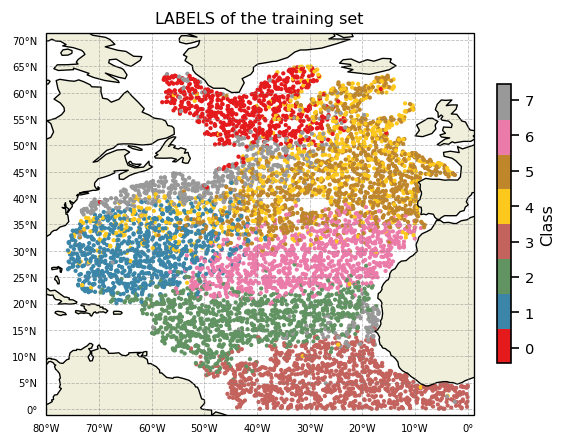
Geographic distribution of classes
Warning
To follow this section you’ll need to have Cartopy installed and working.
A map of labels can now easily be plotted:
[16]:
proj = ccrs.PlateCarree()
subplot_kw={'projection': proj, 'extent': np.array([-80,1,-1,66]) + np.array([-0.1,+0.1,-0.1,+0.1])}
fig, ax = plt.subplots(nrows=1, ncols=1, figsize=(5,5), dpi=120, facecolor='w', edgecolor='k', subplot_kw=subplot_kw)

kmap = m.plot.cmap()
sc = ax.scatter(ds['LONGITUDE'], ds['LATITUDE'], s=3, c=ds['PCM_LABELS'], cmap=kmap, transform=proj, vmin=0, vmax=m.K)
cl = m.plot.colorbar(ax=ax)

gl = m.plot.latlongrid(ax, dx=10)
ax.add_feature(cfeature.LAND)
ax.add_feature(cfeature.COASTLINE)
ax.set_title('LABELS of the training set')
plt.show()
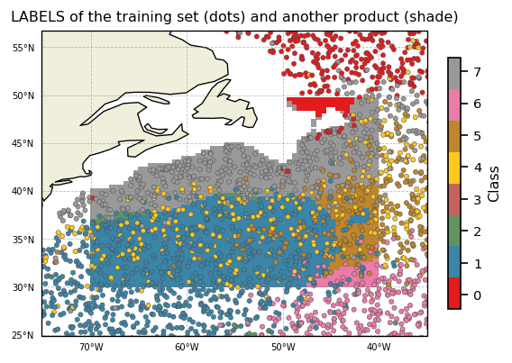
Since we predicted labels for 2 datasets, we can superimpose them
[17]:
proj = ccrs.PlateCarree()
subplot_kw={'projection': proj, 'extent': np.array([-75,-35,25,55]) + np.array([-0.1,+0.1,-0.1,+0.1])}
fig, ax = plt.subplots(nrows=1, ncols=1, figsize=(5,5), dpi=120, facecolor='w', edgecolor='k', subplot_kw=subplot_kw)

kmap = m.plot.cmap()
sc = ax.pcolor(ds_gridded['longitude'], ds_gridded['latitude'], ds_gridded['PCM_LABELS'], cmap=kmap, transform=proj, vmin=0, vmax=m.K)
sc = ax.scatter(ds['LONGITUDE'], ds['LATITUDE'], s=10, c=ds['PCM_LABELS'], cmap=kmap, transform=proj, vmin=0, vmax=m.K, edgecolors=[0.3]*3, linewidths=0.3)
cl = m.plot.colorbar(ax=ax)

gl = m.plot.latlongrid(ax, dx=10)
ax.add_feature(cfeature.LAND)
ax.add_feature(cfeature.COASTLINE)
ax.set_title('LABELS of the training set (dots) and another product (shade)')
plt.show()
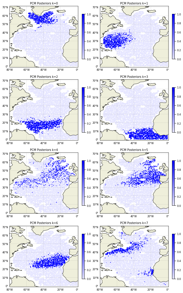
Posteriors are defined for each data point and give the probability of that point to belong to any of the classes. It can be plotted this way:
[18]:
cmap = sns.light_palette("blue", as_cmap=True)
proj = ccrs.PlateCarree()
subplot_kw={'projection': proj, 'extent': np.array([-80,1,-1,66]) + np.array([-0.1,+0.1,-0.1,+0.1])}
fig, ax = m.plot.subplots(figsize=(10,22), maxcols=2, subplot_kw=subplot_kw)

for k in m:
    sc = ax[k].scatter(ds['LONGITUDE'], ds['LATITUDE'], s=3, c=ds['PCM_POST'].sel(pcm_class=k),
                       cmap=cmap, transform=proj, vmin=0, vmax=1)
    cl = plt.colorbar(sc, ax=ax[k], fraction=0.03)
    gl = m.plot.latlongrid(ax[k], fontsize=8, dx=20, dy=10)
    ax[k].add_feature(cfeature.LAND)
    ax[k].add_feature(cfeature.COASTLINE)
    ax[k].set_title('PCM Posteriors k=%i' % k)