Features preprocessing explained
Note
pyXpcm performs automatically all the data preprocessing for you. You should not have to manipulate your data before being able to fit or classify. This page is an explanation of the preprocessing steps performed under the hood by pyXpcm.
The Profile Classification Model (PCM) requires data to be preprocessed in order to match the model vertical axis, to scale feature dimensions with each others and to reduce the dimensionality of the problem. Preprocessing is done internally by pyXpcm. Each step can be parameterised.
The PCM preprocessing operations are organised into 4 steps:
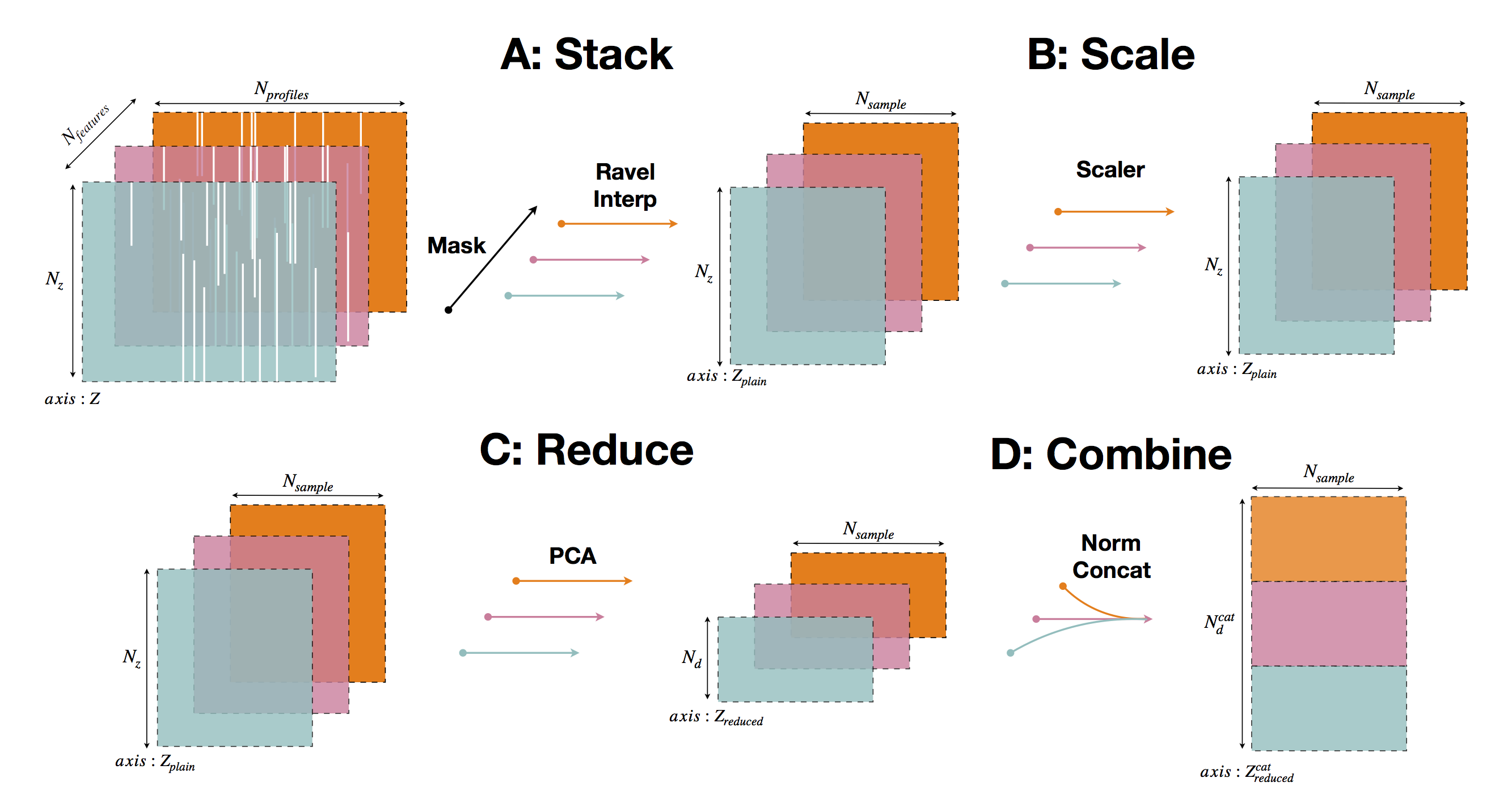
Stack
This step mask, extract, flatten and transform any ND-array set of feature variables (eg: temperature, salinity) into a plain 2D-array collection of vertical profiles usable for machine learning methods.
Mask
This step computes a mask of the input data that will reject all profiles that are full of nans over the depth range of feature vertical axis. This ensure that all feature variables will be successfully retrieved to fill in the plain 2D-array collection of profiles.
This operation is conducted by pyxpcm.xarray.pyXpcmDataSetAccessor.mask(), so that the mask can be computed (and plotted) this way:
[2]:
mask = ds.pyxpcm.mask(m)
print(mask)
<xarray.DataArray 'pcm_MASK' (latitude: 53, longitude: 61)>
dask.array<eq, shape=(53, 61), dtype=bool, chunksize=(53, 61), chunktype=numpy.ndarray>
Coordinates:
  * latitude   (latitude) float32 30.023445 30.455408 ... 49.41288 49.737103
  * longitude  (longitude) float32 -70.0 -69.5 -69.0 -68.5 ... -41.0 -40.5 -40.0
[3]:
mask.plot();

Ravel
For ND-array to be used as a feature, it has to be ravelled, flatten, along the N-1 dimensions that are not the vertical one. This operation will thus transform any ND-array into a 2D-array (sampling and vertical_axis dimensions) and additionnaly drop profiles according to the PCM mask determined above.
This operation is conducted by pyxpcm.pcm.ravel().
The output 2D-array is a xarray.DataArray that can be chunked along the sampling dimension with the PCM constructor option chunk_size:
[4]:
m = pcm(K=3, features=features_pcm, chunk_size=1e3).fit(ds)
By default, chunk_size='auto'.
[5]:
X, z, sampling_dims = m.ravel(ds['TEMP'], dim='depth', feature_name='TEMP')
X
[5]:
- sampling: 2289
- depth: 152
- dask.array<chunksize=(1000, 152), meta=np.ndarray>
Array Chunk Bytes 1.39 MB 608.00 kB Shape (2289, 152) (1000, 152) Count 27 Tasks 3 Chunks Type float32 numpy.ndarray - depth(depth)float32-1.0 -3.0 -5.0 ... -1980.0 -2000.0
- axis :
- Z
- units :
- meters
- positive :
- up
array([-1.00e+00, -3.00e+00, -5.00e+00, -1.00e+01, -1.50e+01, -2.00e+01, -2.50e+01, -3.00e+01, -3.50e+01, -4.00e+01, -4.50e+01, -5.00e+01, -5.50e+01, -6.00e+01, -6.50e+01, -7.00e+01, -7.50e+01, -8.00e+01, -8.50e+01, -9.00e+01, -9.50e+01, -1.00e+02, -1.10e+02, -1.20e+02, -1.30e+02, -1.40e+02, -1.50e+02, -1.60e+02, -1.70e+02, -1.80e+02, -1.90e+02, -2.00e+02, -2.10e+02, -2.20e+02, -2.30e+02, -2.40e+02, -2.50e+02, -2.60e+02, -2.70e+02, -2.80e+02, -2.90e+02, -3.00e+02, -3.10e+02, -3.20e+02, -3.30e+02, -3.40e+02, -3.50e+02, -3.60e+02, -3.70e+02, -3.80e+02, -3.90e+02, -4.00e+02, -4.10e+02, -4.20e+02, -4.30e+02, -4.40e+02, -4.50e+02, -4.60e+02, -4.70e+02, -4.80e+02, -4.90e+02, -5.00e+02, -5.10e+02, -5.20e+02, -5.30e+02, -5.40e+02, -5.50e+02, -5.60e+02, -5.70e+02, -5.80e+02, -5.90e+02, -6.00e+02, -6.10e+02, -6.20e+02, -6.30e+02, -6.40e+02, -6.50e+02, -6.60e+02, -6.70e+02, -6.80e+02, -6.90e+02, -7.00e+02, -7.10e+02, -7.20e+02, -7.30e+02, -7.40e+02, -7.50e+02, -7.60e+02, -7.70e+02, -7.80e+02, -7.90e+02, -8.00e+02, -8.20e+02, -8.40e+02, -8.60e+02, -8.80e+02, -9.00e+02, -9.20e+02, -9.40e+02, -9.60e+02, -9.80e+02, -1.00e+03, -1.02e+03, -1.04e+03, -1.06e+03, -1.08e+03, -1.10e+03, -1.12e+03, -1.14e+03, -1.16e+03, -1.18e+03, -1.20e+03, -1.22e+03, -1.24e+03, -1.26e+03, -1.28e+03, -1.30e+03, -1.32e+03, -1.34e+03, -1.36e+03, -1.38e+03, -1.40e+03, -1.42e+03, -1.44e+03, -1.46e+03, -1.48e+03, -1.50e+03, -1.52e+03, -1.54e+03, -1.56e+03, -1.58e+03, -1.60e+03, -1.62e+03, -1.64e+03, -1.66e+03, -1.68e+03, -1.70e+03, -1.72e+03, -1.74e+03, -1.76e+03, -1.78e+03, -1.80e+03, -1.82e+03, -1.84e+03, -1.86e+03, -1.88e+03, -1.90e+03, -1.92e+03, -1.94e+03, -1.96e+03, -1.98e+03, -2.00e+03], dtype=float32) - sampling(sampling)MultiIndex(latitude, longitude)
array([(30.02344512939453, -70.0), (30.02344512939453, -69.5), (30.02344512939453, -69.0), ..., (49.73710250854492, -41.0), (49.73710250854492, -40.5), (49.73710250854492, -40.0)], dtype=object) - latitude(sampling)float6430.02 30.02 30.02 ... 49.74 49.74
array([30.023445, 30.023445, 30.023445, ..., 49.737103, 49.737103, 49.737103])
- longitude(sampling)float64-70.0 -69.5 -69.0 ... -40.5 -40.0
array([-70. , -69.5, -69. , ..., -41. , -40.5, -40. ])
- long_name :
- Temperature
- standard_name :
- sea_water_temperature
- units :
- degree_Celsius
- valid_min :
- -23000
- valid_max :
- 20000
See the chunksize of the dask.array.Array for this feature.
Interpolate
Even if input data vertical axis are in the range of the PCM feature axis, they may not be defined on similar level values. In this step, if the input data are not defined on the same vertical axis as the PCM, an interpolation is triggered. The interpolation is conducted following these rules:
If PCM axis levels are found into the input data vertical axis, then a simple intersection is used.
If PCM axis starts at the surface (0 value) and not the input data, the 1st non-nan value is replicated to the surface, as a mixed layer.
If PCM axis levels are not in the input data vertical axis, a linear interpolation through the
xarray.DataArray.interp()method is triggered for each profiles.
The entire interpolation processed is managed by a pyxpcm.utils.Vertical_Interpolator instance that is created at the time of PCM instanciation.
Scale
Each variable can be normalised along a vertical level. This step ensures that structures/patterns located at depth in the profile, will be considered similarly to those close to the surface by the classifier.
Scaling is defined at the PCM creation (pyxpcm.models.pcm) with the option scale. It is an integer value with the following meaning:
0: No scaling
1: Center on sample mean and scale by sample std
2: Center on sample mean only
Recuce
[TBC]
Combine
[TBC]